Calculational Mathematics and CalcCheck
Reference Material
| PDF “2DM3CheatSheet” | Short 4 page summary of core material; uses informal names. |
| HTML Theorem List | Uses CalcCheck names and refers to specific homework and exercises. |
Videos
Introduction to Discrete & Calculational Maths Sep 8
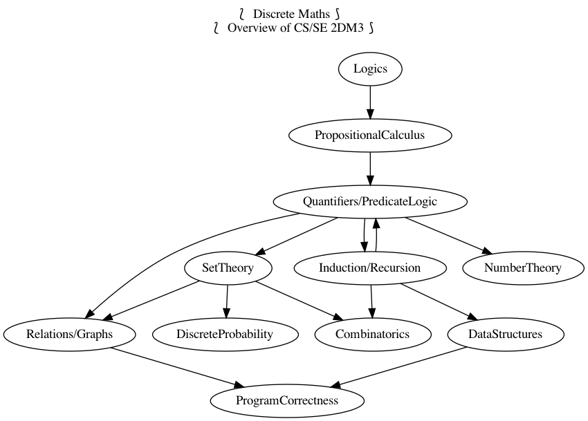
What is a calculational proof? What is discrete mathematics? How is math related to programming: “proofs-as-programs”.
Grammatical Analysis and Boolean Operators Sep 10
A proof is a “story”, and calculation hints are the “transitions” that make the story flow nicely. The formulae are the “sentences” and they are formed from operators, constants, and variables which act as “verbs”, “names”, and “pronouns”, respectively.
ℕumber arithmetic is learned by memorising parts of infinitely large addition and multiplication tables. In contrast, 𝔹oolean arithmetic has tiny 2×2 “truth tables”. As such, 𝔹 may be easier to learn than ℕ.
Ladies and Tigers, a teaser Sep 11
Continuing the discussion on Boolean operators and how they can be used to model puzzles.
Substitution Sep 15
Textual substitution is a way to implement function application, grafting on trees, and can be used for assignment commands in programming.
Inference rules, Proofs-are-programs, and Equivalence Part I Sep 17
Update: There will be no knights and knaves problems in the upcoming Sep 22 midterm; but possibly in a future midterm.
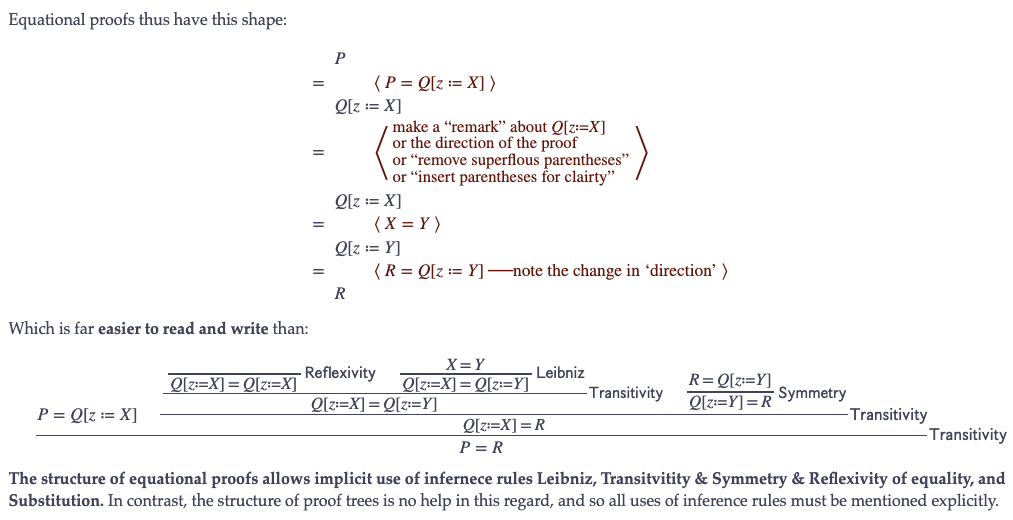
The inference rules act as the foundational justification for the equational proof style; the online lecture notes go into more detail.
Inference rules, Proofs-are-programs, and Equivalence Part II (with lofi music) Sep 18
Quickly show how a program can be shown to meet its specification, discuss equivalence and negation for the purposes of solving knights and knaves problems.
Sep 22 is the first midterm; it is online during class time.
Tabulation vs Calculation Sep 24
We review basic operations on the Booleans with a focus on how manipulating symbols can be more effective than constructing truth tables, or evaluating expressions by “plug and chug” simplifications.
We also discuss formalisations of English phrases as propositional expressions.
The Unfold-fold Heuristic and Induction Sep 25
When a new operation is introduced, one can reason about it by using its definition to ‘see’ familiar operation, manipulate those, then invoke the definition to ‘fold-up’.
To show a property P(n) ranging over natural numbers n : ℕ, it is not reasonable to evaluate P at the infinitely many possible values for n. Instead one uses mathematical induction.
Conjunction Sep 29
Starting from the Golden Rule, as a definition of conjunction, we see how to derive a few properties of ∧ then move on to consider examples involving Ladies and Tigers. We wrap up with a brief look at induction.
Induction Oct 1
We consider a few inductively defined functions and prove properties about them. Of note is ‘monus’, subtraction, which is defined inductively on multiple arguments. Then, we consider a few ‘advanced’ implication theorems.
Replacement Oct 2
With implication in-hand, we can express the Leibniz inference rule as an axiom —the notes contain a discussion on the relationship between inference rules and axioms.
Continuing with the assignments on Order Theory, we discuss how implication is itself an order —as well as an operation— on the 𝔹ooleans.
Oct 6 is the second midterm; it is online during class time.
Quantification/Loops and Extended Proof Style Oct 8 with “playground”
Quantification is a mathematical abstraction of loops:
int s = 0; for(int i = a; i != b; i++){s += f(i);}is an implementation of the quantification(∑ i : ℤ ❙ a ≤ i ≠ b • f i).We also discuss how transitivity can be used to extend the calculational proof style with other relations besides equality.
Proof Techniques and Relaxed Proof Style Oct 9
We review how CalcCheck permits relaxed proofs such as `with` for modus ponens and `Assuming` for implication introduction.
We also quickly discuss `Using`, which is a way to use theorems as proof techniques!
Oct 9 to Oct 16 Reading Week, no classes.
Quantification with ΣΠ∀∃ and Scope Oct 20
Quickly review basics of quantifiers and their implementations, loops; then introduce ∃/∀ as quantifiers (loops, iterations) for ∨/∧; then wrap up with the notion of scopes via examples of names in friend groups.
- Midterm Prep: In-depth “Assuming” and some “∀” Oct 22
Theorem Statements Suggest Proof Structure (•̀ᴗ•́)و Oct 23
We review, compare, and contrast proving theorems directly versus using a relaxed proof style. Textual substitution on quantifiers is also reviewed briefly.
Oct 27 is the third midterm; it is online during class time and the ‘Midterm Prep’ was created to, well, prepare you for the midterm.
Feedback Replies & Quantification Oct 29
Let's discuss the entries posted on the feedback channel as well as impressions of the previous midterm. Then let's continue with Quantification and it's possible implementations via loops.
Monotonicity: From ∧/∨ to ∀/∃ Nov 3
We discuss order preservation rules then move on to talk about (general) induction and how it can be invoked with CalcCheck's “Using” mechanism —which allows a theorem to be used as a proof technique.
Sequences and Induction Nov 5
The idea behind induction is that if a property holds for atomic constructions and the property is preserved by compound constructions then —since everything under consideration is formed from these possible constructions— everything has the property begin discussed.
Incidentally, induction can also be phrased more compactly as follows: Predicates starting at ‘true’ and preserving truth, are constantly ‘true’: Suppose \(P : τ → 𝔹\) is a predicate on an ordered space, then \[P\, ⊥ \;∧\; (∀ x,y : τ \,❙\, x ⊑ y • P\, x \,⇒\, P\, y) \;⇒\; (∀ x : τ • P\, x) \]
“Typed” Set Theory 𝑰 Nov 6
Sets are like any other data structure, such as ℕumbers or sequences. However, there is a particular ‘reflection’ of types-as-sets: Every type is a set, but not the other way around. ( Likewise, every sequence yields a set, but no canonical choice the other way around. )
Types make sure things don't go wrong, such as multiplying a set by a letter!
Nov 10 is the fourth midterm; it is online during class time.
“Typed” Set Theory 𝑰𝑰 Nov 12
Continuing part 𝑰.
Cartesian Products, a theory of records Nov 13
We look at Cartesian Products and projections, which can be thought of as the mathematical underpinning of “records/classes and fields” found in programming.
We also quickly take a look at Currying —yet another instance of the “Programming ≈ Proving” slogan repeated throughout these lectures.
Finally, we consider sets of pairs, ‘relations’, as a form of non-deterministic computing.
A ‘Brutal’ Introduction to Relations Nov 17
We conclude Set Theory with an example of “division of sets” known as the pseudo-complement: We show how it's defining universal property can be used to calculate an explicit definition. Assuming ⊆ and ∈, the same idea applies to other concepts defined by universal properties, such as ╱, ╲, ∪, ∩, and -.
Next, we look at specific kinds of sets, namely sets of pairs. Just as sets “hide singe quantified variables” involving ∀ via = and ⊆, and hide ∃ via ∈; relations allows us to “hide two quantified variables”. More generally, “n-ary relations” with n = 0 are propositions, n = 1 are predicates/sets, and with n = 2 are simple relations, as shown here.
Compare with “A ‘Gentle’ Introduction to Relations (Nov 19)”.
A ‘Gentle’ Introduction to Relations Nov 19
Relations are just sets of pairs, but there are interesting interpretations of such sets: Matrices, Graphs, Programs. As such, there are interesting operations on these particular kinds of sets such as converse and composition.
Operations on relations, such as composition, “hide quantified dummy variables” and so “wide, lengthy, statements” take on more compact forms. A useful law involving quantifier-free calculations is the Dedekind rule and the Modal laws. An example involving the distributivity of univalent relations over intersection is shown.
Compare with “A ‘Brutal’ Introduction to Relations (Nov 17)”.
Wrapping up Relations Nov 20
Concluding our discussion on relations by considering how “relation division” appears —either the shape of residuals “R ╱ S” or via converse “R ⨾ S˘” and the Modal & Dedekind rules.
We then look at how this allows us to read the Z ISO standard, and begin combinatorics by counting the size of certain kinds of arrows.
Nov 24 is the fifth midterm; it is online during class time.
ISO Z Standard & Combinatorics Nov 26
Since Midterm 5 showed that not everyone is very comfortable with relations, the plan is not to “bulldoze onward” to new material but instead to “ping-pong” between new material, and to connect it back to relations to reinforce the concepts therein. A few fun graphs are shown.
Sequences vs Sets vs Bags
- Sequence: [x₀, x₁, …, xₙ] … order and multiplicity matter
- Set : {x₀, x₁, …, xₙ} … neither order nor multiplicity matter
- Bag : ⦃x₀, x₁, …, xₙ⦄ or ⟅x₀, …, xₙ⟆ order doesn't matter but multiplicity does
- Sets ≈ exitence is enough …. “∈” is the key!!
- Bags ≈ I need to know which one … “♯” “how many times is it there?”
- Bags ≈ multi-relations = multi-sets
Multirelations! Nov 27
We speak of people in Toronto sharing the same number of hair, multiple edges in a graph, and how bags account for “mor information” by yielding the number of times an element occurs whereas sets only care “whether it's there or not” —this is reminicient of classical vs constructive maths. A few fun graphs are shown.
Reachability Dec 1
We quickly review bags —multisets— and then talk about closures, which capture the idea of “add just enough so the result has the deisred property”. This then leads us to talk about transitive closures which can be used to to elegantly express proeprties on graphs that would otherwise be a nightmare to work with (if quantifiers, ∀∃, were used).
Trees Dec 3
Directed, acyclic, connected graphs are known as trees. They have the particular property that they can be expressed as inductive data types: Whereas a sequence is either empty ε or has a right-child
x ◁ r, a tree is either empty ◬ or has two childrenl ◿ x ◺ r. We also look at other examples of inductively defined structures and briefly mention topological sort.Wrapping up the term: Closures, Topological Sort, Probability Theory Dec 4
We finish the discussion on closures and kerneal that was started last time. We look at DAGs and how they allow ‘sharing’ of structure and how we can traverse graphs: We show visitation and topological sorting. Finally, we wrap up with a terse introduction to probability theory as “Σ in disguise” and close with inference rules/trees and structural induction (•̀ᴗ•́)و
Closing off with some induction example in Agda Dec 8
All the best with exams!
| ⇨ Github Repository ⇦ |